Descriptive Statistics in Six Sigma plays an important role. But, if we do not display that data in a way that can be easily understood, then it becomes useless to us or, worst yet, we might draw the wrong conclusions from it.
In this module, we discuss Descriptive Statistics as used in the Measure Phase of Six Sigma. We’ll go through the key measures that describe key characteristics of variation in a data set.
Descriptive Statistics includes measures of location and measures of dispersion.
Measures of Location
Measures of Location is formally called measures of central tendency. For this type of descriptive statistic, we are mostly interested in the Mean, Median, and the Mode.
Mean
In a data set, measures of central tendency is a way to represent the central value in a collection of data. The basic name for this value is The Mean, often times called X-Bar.
The Mean is the sum total of all the data values divided by the number of data points. You know this value by its common name – the average.
Median
The Median is the midpoint or the middle value when the data is arranged from smallest to largest. For an even set of data, the Median is the average of the middle two values.
For example, take the data set below:
3, 5, 7, 12, 13, 14, 21, 23, 23, 23, 23, 29, 40, 56
Because this data set is even, the middle two numbers can be added and then divided by two to arrive at the average, which will be our median:
21 + 23 = 44
44 / 2 = 22 is the Median.
Mode
The Mode is the most frequently occurring number in a data set. For example, consider the data set below:
3, 5, 7, 12, 13, 14, 20, 23, 23, 23, 23, 29, 39, 40, 56
In this data set that is sorted from smallest to largest, 23 occurs four times, which is the most frequent occurring number and, hence, 23 is the mode in this data set.
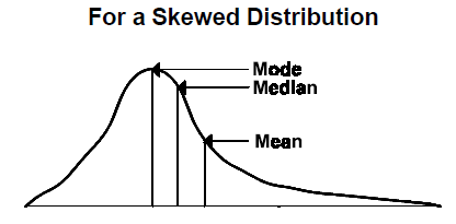
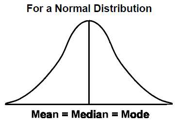
If the data set is normally distributed, then the Mean = Median = Mode like the following:
Measures of Dispersion
For smaller data sets, the Range and Interquartile Range are good measures that indicate variability in the data set.
To see the spread of a data set, we are mostly interested in the dispersion of the data. For this, we are curious about the Range, Interquartile Range, Standard Deviation, and the Variance.
Range
The range in descriptive statistics is the difference between the largest observation and the smallest observation in the data set.
Range = Max – Min
A small range would indicate a small amount of variability. A large range would indicate a large amount of variability.
Interquartile Range
The Interquartile Range is the difference between the 75th percentile and the 25th percentile.
IQR = Q3 – Q1
When your data looks skewed, the Range and IQR are good quick indicators that tell you something about the variability in the data set.
As the data set gets larger, however, the standard deviation becomes a more reliable measure of variability.
Standard Deviation
The Standard Deviation, or Sigma, is the average deviation of values from the mean of a given data set. Simply, it’s the average spread from the mean.
Variance
The variance is the average squared deviation of each individual data point from the mean.
Let’s Do An Example
Let’s go through an example that demonstrates the Mean, Variance, and Standard Deviation.
Suppose you measured several dogs at the park. Below are the heights of the dogs in millimeters:
- 600
- 470
- 170
- 430
- 300
To get the Mean,
600+470+170+430+300 = 1970
Mean = 1970 /5 = 394
Now, let’s calculate the Variance. First, we need to calculate the difference or each dog’s height from the Mean.
- 600-394 = 206
- 470-394 = 76
- 170-394 = -224
- 430-394 =36
- 300-394 = -94
Now, we square each of the sums above like so:
Variance = [206^2 + 76^2 + (-224)^2 + 36^2 +(-94)^2] / 5 = 21704
To get the Standard Deviation, we only need to square root the variance:
SQRT(21704) = 147
Up Next
Next, we’ll discuss the various distributions commonly used by Six Sigma Black Belts in DMAIC Projects.
[contentblock id=16 img=gcb.png]


Comments are disabled for this post.